Understanding the Superset Semantic Layer

Intro to the Semantic Layer

Apache Superset has grown to become one of the most popular business intelligence platforms out there because of the rich feature set that is available in an accessible, open source package. One of the tentpole feature areas in Superset is the semantic layer.

A semantic layer is an abstraction over your base data that lives in your data warehouse or data lake. The semantic model maps SQL to more human-friendly metaphors.

The Superset community didn't invent the semantic layer of course. It was supposedly first patented by BusinessObjects in 1992 and slowly incorporated into other legacy data science tools like Cognos and Microstrategy. More recently, Looker (which was acquired by Google Cloud) built an entire product essentially around a semantic layer (LookML). Looker’s LookML brought the semantic layer idea to the forefront of the BI discussion.

After a decade of acquisitions in the BI space, Apache Superset remains one of the few open-source BI tools left with a semantic layer. Let's now dive in to understand Superset's flavor of the semantic layer.

Thin or Thick Semantic Layer?

The semantic layer in Superset is pretty thin by design. Why is this?

The last generation of BI tools like Looker encouraged end-users to invest heavily in building out tons of LookML models to populate the semantic layer. While this established Looker as a source of truth in an organization for business metrics, it also created an immense amount of lock in in your BI tool. You couldn’t take your LookML models with you and use them with another tool, if you decided to switch BI tools. Google’s acquisition of Looker accelerated organizations’ anxieties around this lock-in, to the point that Google actually was forced to integrate LookML with Tableau. This way, organizations could use LookML for transformation (Looker’s strength) and Tableau for visualization (Tableaus’ strength).

The future however is looking to be very different from the past. There are now entire open source projects and products building unified semantic layers, to sit between the database and the BI layer:

• Cube
• MetriQL
• Transform
• and many others!

The goal of a thin semantic layer then is to primarily enable last mile data transformation for the explicit purpose of visualization in your BI tool. I’ll showcase some concrete examples throughout this post.

Now that I’ve set the stage with some context, let’s dive into the specifics. The semantic layer in Superset consists of three main metaphors:

• Virtual Datasets
• Metrics
• Calculated Columns

As you traverse through this blog post, it’s helpful to remember that all of these features exist to help you craft better and more complex SQL queries. BI tools provide convenient UI interfaces and affordances so you can avoid having to manually write very long SQL queries from scratch.

Physical vs Virtual Datasets

The data layer in Superset falls into two buckets: physical datasets and virtual datasets.

A physical dataset in Superset represents a table or view in your database. Because a physical dataset reflects a real, physical table, Superset is able to automatically pull in relevant information from the database (like schema and column types). This information is saved in Superset’s metadata database. If a change to the underlying database table occurs, you can click Sync Columns from Source to force Superset to update its internal data model.

Virtual datasets enable you to elevate a freeform SQL query against your database into a dataset entity in Superset. Virtual datasets inherit most of the same superpowers as physical datasets:

• column types (inferred from results of running the query)
• ability to define metrics
• ability to define calculated columns
• ability to certify metrics or calculated columns
• setting a cache timeout

Using Virtual Datasets

The fastest way to create a virtual dataset is to write and run your query in SQL Lab. Then, you can click Explore near the results tray and you’ll be asked to name the virtual dataset:

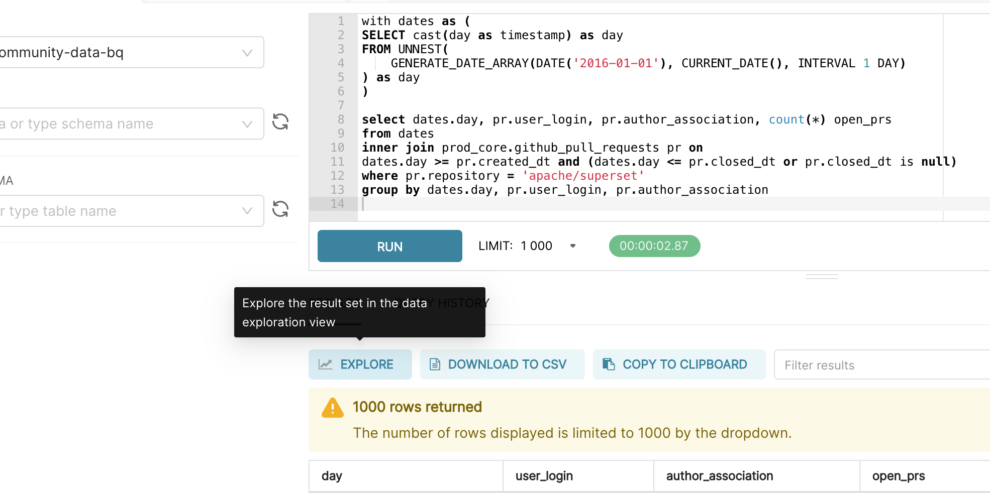
So when should you use a virtual dataset? Here are some use cases with some concrete examples.

1. Joining multiple tables (or self-joining against the same table)
   • To visualize total revenue by customer persona, we need to JOIN between a customers table and a orders table to form the customers_orders virtual dataset.
2. Ad-hoc, one-off exploratory analysis
   • If you want to quickly launch an Explore workflow from the results of a custom SQL query you wrote in SQL Lab, you need to first save the query as a virtual dataset.
3. Transforming data in more nuanced ways than currently what Explore
   • No-code UI’s can’t really replace the need to write custom SQL entirely because of the complexity, but Superset’s Explore view attempts to augment common slice-and-dice workflows common in analytics. For example, if you want to heavily transform the underlying data using window functions, virtual datasets are a great way to prep the data before visualizing in Explore.

You’ll notice that some of these workflows have a “temporary” framing attached to them. This is because populating the semantic layer with hundreds or even thousands of virtual datasets makes it more difficult for a data platform / governance team to help keep the backend data systems (databases, data pipelines, caching layers, etc.) highly performant and reliable. In addition, in larger organizations, this can lead to data drift & metric inconsistency.

But as with most advice, it’s contextual to your organization! If you’re a small, nimble team like us at Preset, virtual datasets are powerful at unblocking end-user analysts in the short run. Commonly used transformations in the semantic layer can then be methodically be migrated to the data pipeline over time, in a more agile way.

Metrics

Superset’s origins are in fast, slice & dice, exploratory analytics specifically for Apache Druid. In this workflow, it’s natural to alternate between:

• prototyping visualizations quickly using different metrics
• defining a set of commonly used metrics for wider use in an organization

In more specific terms, a metric in Superset is any valid, aggregating SQL snippet that can be included in a SELECT clause. Each line within the SELECT clause below are valid metrics in Superset:

SELECT 
	COUNT(*),
	SUM(CASE WHEN action='deal_closed' THEN 1 ELSE 0 END),
	MAX('revenue'),
	SUM('deals_open') / SUM('deals_closed')
	MAX('revenue') - MIN('revenue')

Here are some use cases:

1. Converting a text / categorical value to an integer, for visualization:

   SUM(CASE WHEN action='deal_closed' THEN 1 ELSE 0 END)

2. Computing a ratio of deals open to deals closed:

   	SUM('deals_open') / SUM('deals_closed')

3. Calculating the range for a column:

   MAX('revenue') - MIN('revenue')

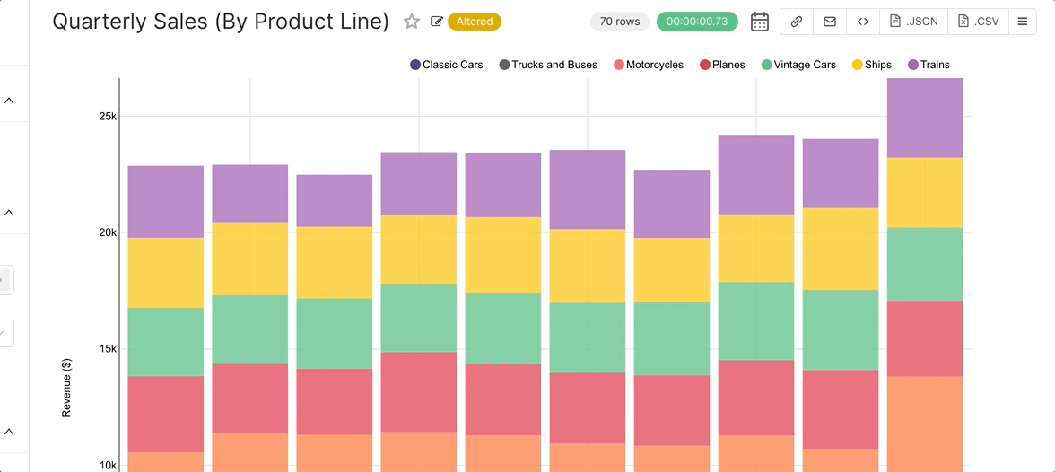
The easiest way to get started with metrics is to select a Time-series visualization type while in the Explore workflow. Then, you can quickly try a few different metrics.

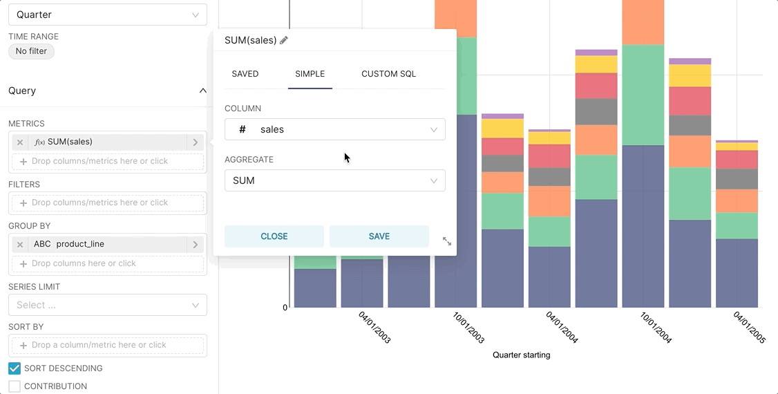
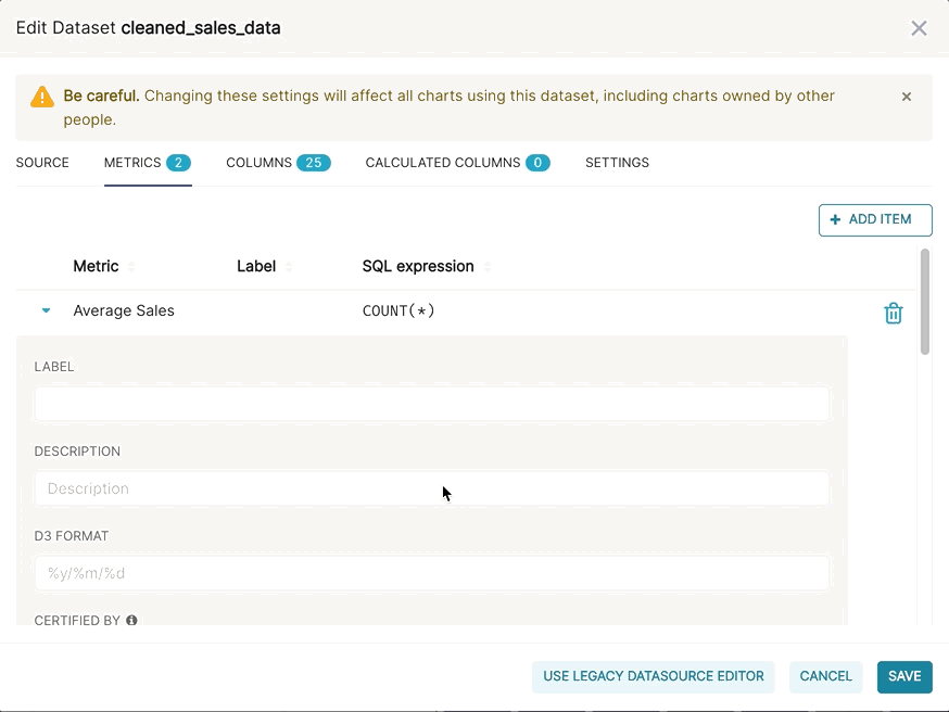
Then, if you want to publish a metric for more common use, you can persist the metric in the Edit Dataset view.

Calculated Columns

Calculated columns let you define simple transformations (as SELECT statements) for quick, last-mile data preparation.

You can define any valid, non-aggregate SQL snippets that can be included in a SELECT clause. Note that this means you can reference multiple columns in your calculated column queries.

Here are some examples:

1. To create a Table chart with clickable links, you can use a calculated column to augment the underlying data with HTML. The following snippet performs string concatenation to generate HTML using each row’s value for repo, parent_id, and title:

   CONCAT('<a href="https://github.com/", repo, '/issues', parent_id, ">', title, '</a>')

2. For a more human-friendly presentation in visualizations, you often want to re-label group names in your data.

   Case 
       When is_purchased is 0 then 'No'
       When is_purchased is 1 then 'Yes'
       Else 'N/A’
   End

3. Converting / casting column types

   CAST(sales_cts) as int)

4. Calculating number of days between two date columns

   DATE_DIFF(DATE '2010-07-07', DATE '2008-12-25', DAY)

Debugging Queries

Ultimately, the end-user facing features of Superset (like the ones discussed in this post) help you generate more complex SQL queries.

• Virtual datasets, metrics, and calculated columns provide useful abstractions and superpowers to augment your queries.
• Explore provides a no-code, drag & drop UI for quickly generating queries that power visualizations.

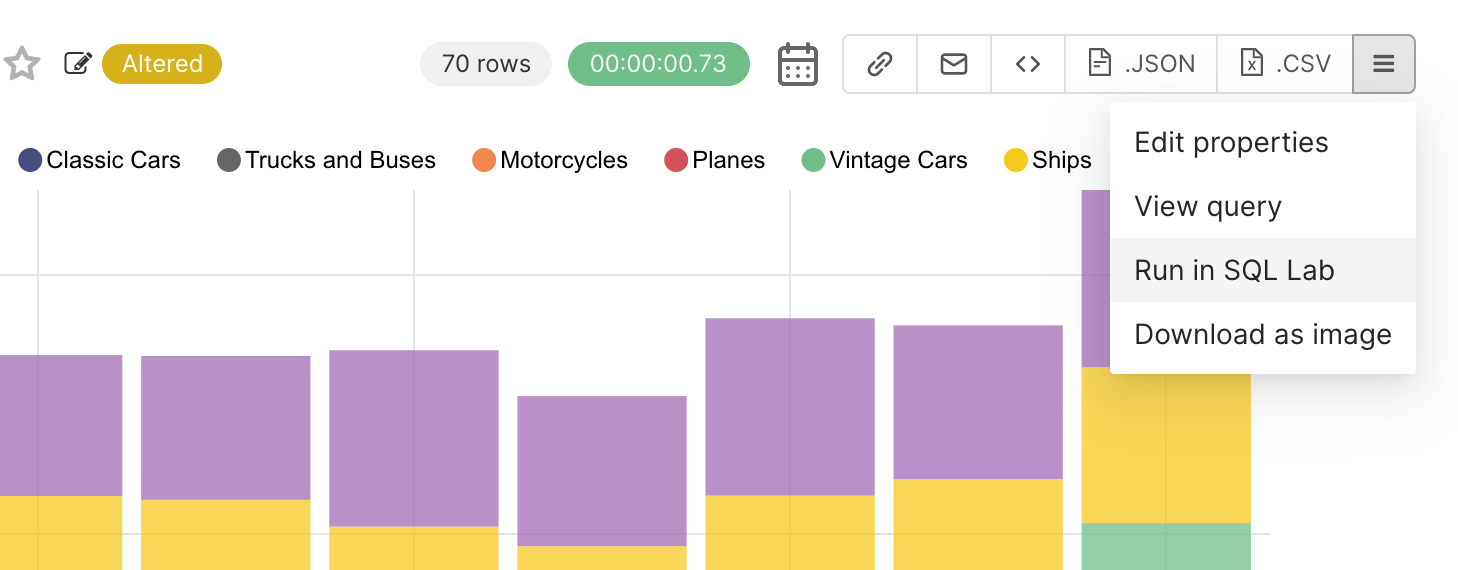
Because the final artifact of the workflows in Superset is SQL, you can use SQL Lab to debug any of the queries that are written. When in Explore, select the hamburger menu in the top right corner and then select View Query to observe the query Superset generated. You can then copy, paste, and run the the query in SQL Lab (make sure you’ve selected the right database context from the drop-down menu while in SQL Lab).

An even faster method is to click Run in SQL Lab from the hamburger menu.

From here, you can:

• Inspect and internalize the shape of complex data, so you can discover what changes in your assumptions you may need to make
• Debug SQL query issues and update the relevant virtual dataset, metric, or calculated column

We'll end this post by mentioning the Semantic Layer documentation in our Preset Docs, which acts as a solid reference & complement to this post.