A Case Study in Dataset-Centric Visualization Using dbt and Snowflake

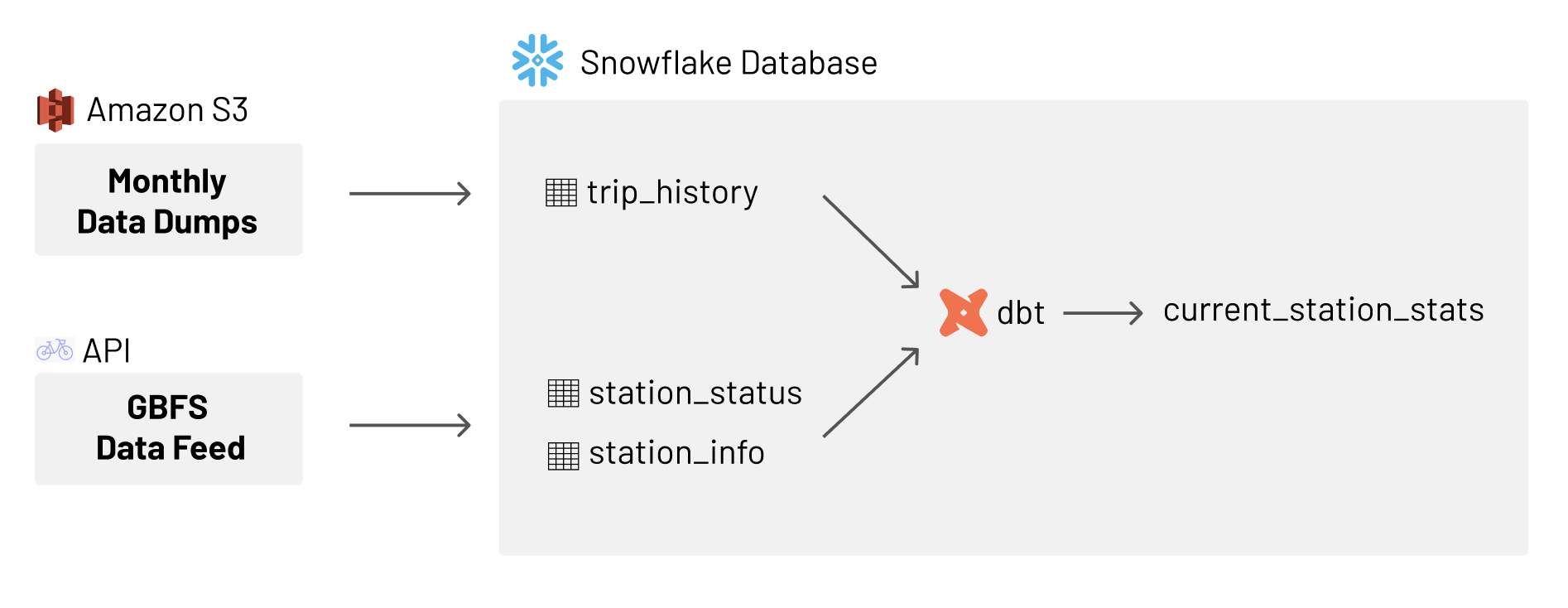
In a previous post, The Case for Dataset-Centric Visualization, Max Beauchemin wrote in-depth about the dataset-centric approach to visualization that’s core to Superset. The graphic from that post below provides a good way to visualize the architecture and flow of the data from database to visualization layer, and allows us to get a high level overview of each of the approaches!

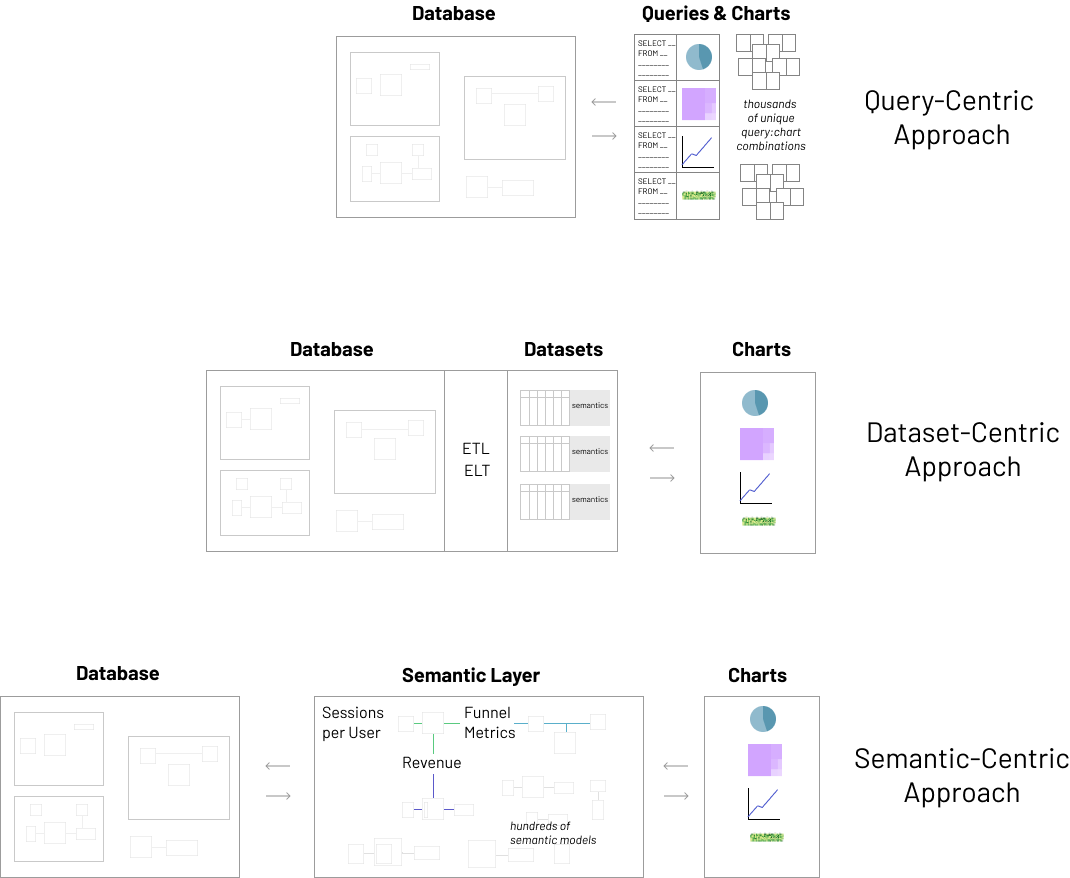
Max goes into extensive detail of the trade-offs that the semantic-centric and query-centric approaches both make, so you can read that for a better understanding of the three approaches.

While Superset does have a semantic layer, it’s deliberately very thin (Understanding the Superset Semantic Layer) and aligns with the dataset centric visualization philosophy!

In this post, I’ll be sharing a case study in applying the dataset-centric visualization approach using real datasets in the hopes it can be a helpful reference for users of both Apache Superset and Preset Cloud.

Introduction to the Datasets

Each different bikeshare program publishes their trip history in varying cadences. In this post we will focus on Citi Bike (the primary bike share system in NYC) and the datasets they provide: their publicly available trip data and their real-time system data in General Bikeshare Feed Specification format.

Trip History

The trip data files contain one record for each ride, around two million records per month, depending on the season. It’s a traditional bike share system with fixed stations where a user picks up a bike at one dock, using a key fob or a code, and returns it at another. The station and time when the ride started and stopped is recorded for each ride.

This data is available in a public s3 bucket:

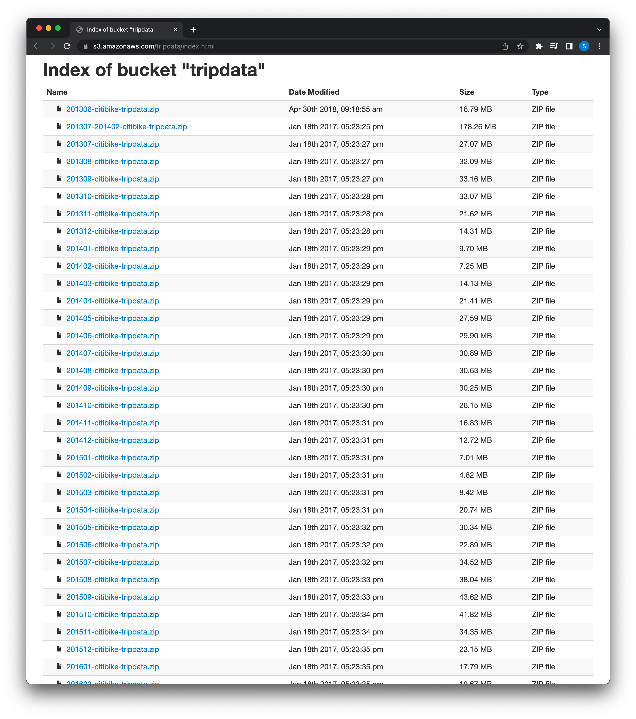
Rider specific information — whether the rider is a subscriber or not — is also provided in the trip history snapshots.
The snapshot data is provided with a schema meant to answer questions like:

• Where do Citi Bikers ride?
• When do they ride?
• How far do they go?
• Which stations are most popular?
• What days of the week are most rides taken on?

And dashboards to visualize and dig deeper into questions like this can be created, for example:

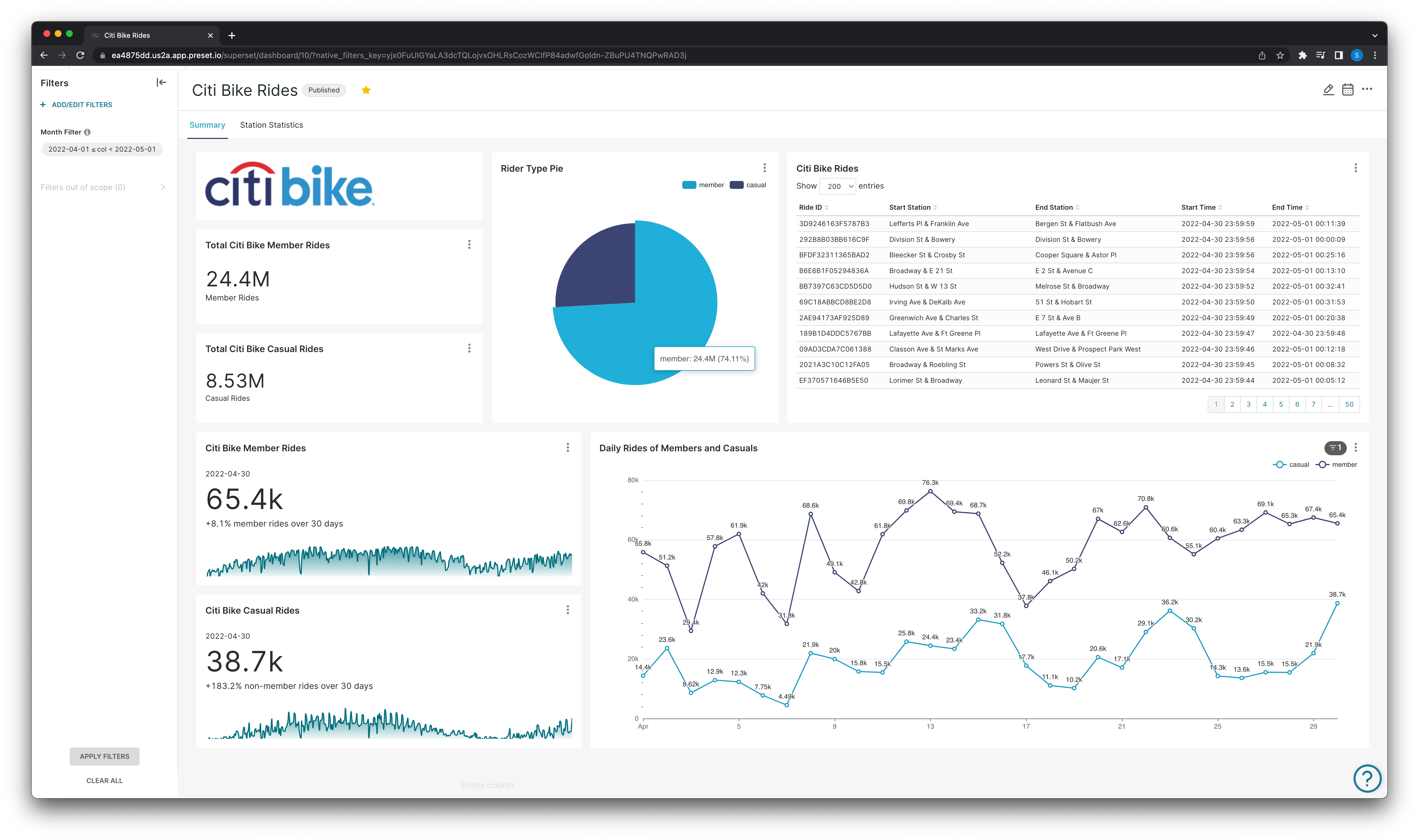
The above is a dashboard made to specifically look into the trip history of subscribers and non-subscribers and understand their general bike usage.

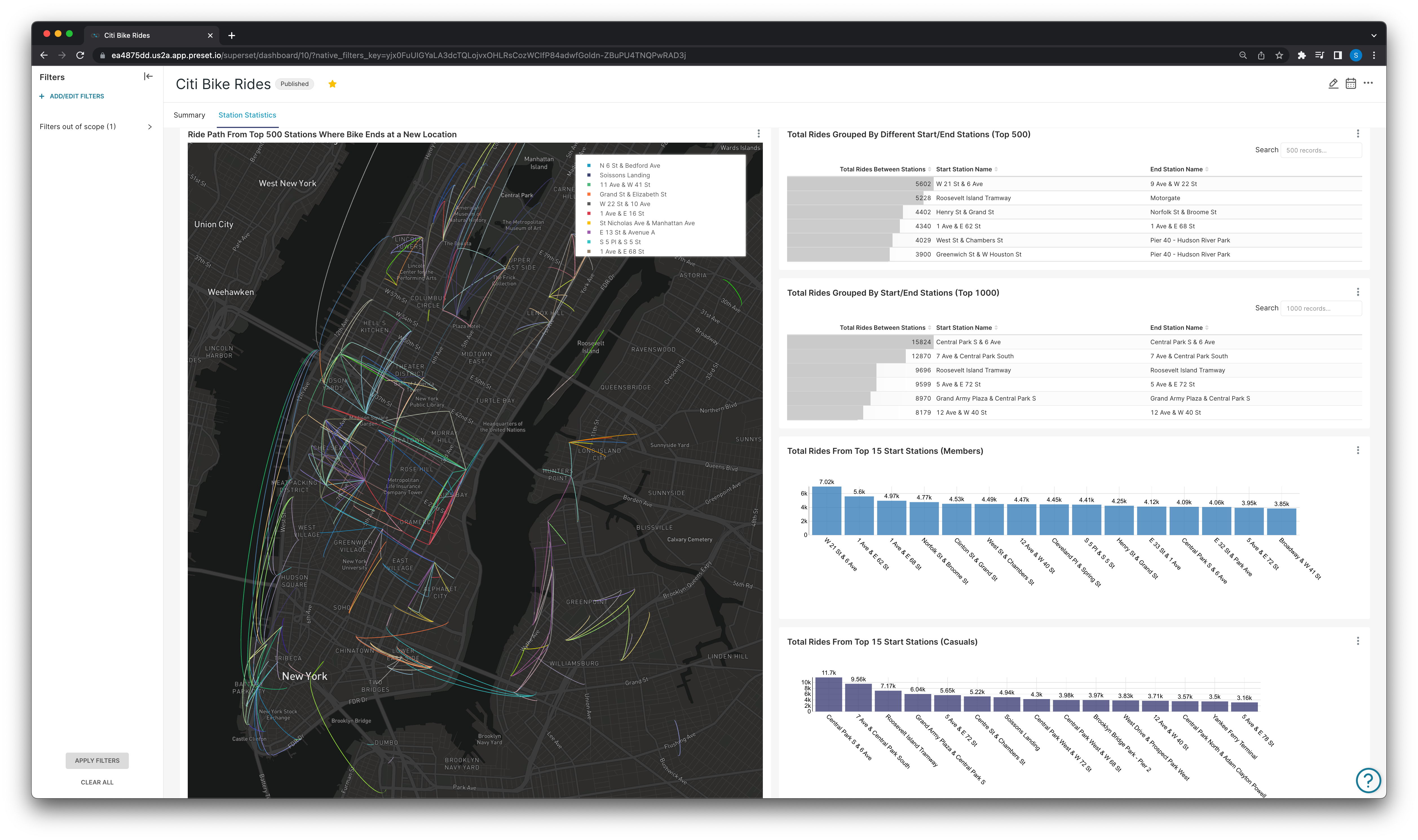
And another can be made to visualize trip statistics between stations for all riders, or ride metrics between stations on a subscriber vs non subscriber basis.

While historical analysis is useful, the clear limitation here is we are limited to analyzing trip history only to the last day of the previous month. The bikeshare dataset gives us an opportunity to use a dataset-centric approach to modeling our data into a “derived” dataset augmented with extra semantics to visualize information beyond the limit of the historical snapshots.

Enrichment with dbt and Dataset-Centric Philosophy

All of the visualizations above are made possible due to the fact that “raw” historical trip data is already provided in a highly normalized fashion with a schema specifically designed to be able to answer the interesting questions in a visual manner. There is a an obvious drawback here — what about station statistics or trip data today?

The snapshots are normalized in a way to allow us to create the dashboards in the previous section. Normalization is generally considered a best practice for developing clean data. Diving deeper, the meaning or goal of data normalization is two-fold:

• Data normalization is the organization of data to appear similar across all records and fields.
• It increases the cohesion of entry types leading to cleansing, lead generation, segmentation, and higher quality data.

Simply put, this process includes eliminating unstructured data and redundancy (duplicates) in order to ensure logical data storage. When data normalization is done correctly, you will end up with standardized information entry. For example, this process applies to how URLs, contact names, street addresses, phone numbers, and even codes are recorded. These standardized information fields can then be grouped and read swiftly.

Dataset-Centric Philosophy

In a dataset-centric approach to modeling, normalizing the raw data is very important because a well normalized dataset can be used to “derive” richer datasets with extra semantics. Datasets for visualization should be augmented with extra semantics to make them valuable for analysis and visualization. By creating derived datasets which incorporate aggregate metric calculations earlier in the ETL/ELT process before surfacing for visualization, many of the issues with change management, maintenance, logic re-use within dashboards, etc. are significantly reduced for a better experience! dbt is the perfect tool to model this data with the dataset-centric approach that helps Superset shine. For those unfamiliar, dbt is a development framework that combines modular SQL with software engineering best practices to make data transformation reliable, fast, and fun.

The content below will focus on how we modeled in the GBFS data and created a derived dataset that will allow us to visualize a bar graph of total rides from a station beyond the last date of the previous month.

General Architecture to Visualize with Real Time Data

With this architecture in place we can now visualize ride metrics to whenever the feed was last ingested:

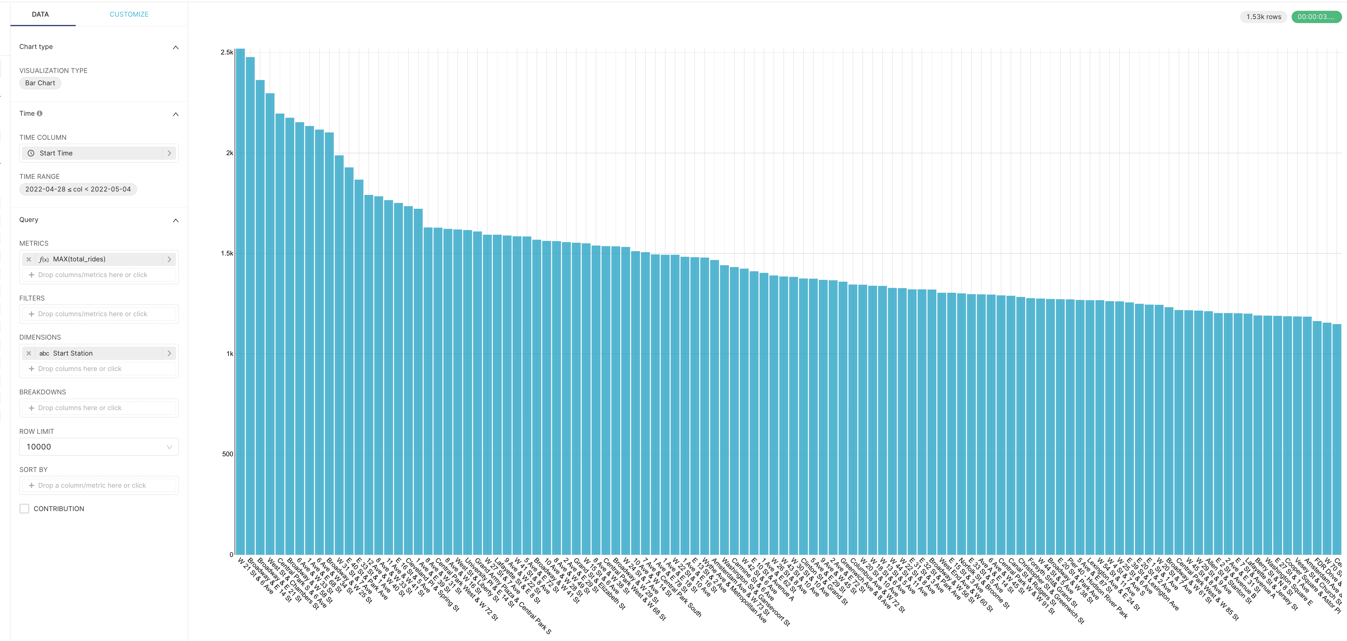
Here we have configured and visualized the total rides in a weekly time-frame using our derived dataset — with three days of total ride history coming from the historical data and four days beyond the last date from the snapshots! This was done without being provided the unique ride IDs that are provided in the historical data which means we can’t analyze this on a subscriber/non-subscriber basis (this is also only added in the historical dataset) but we can get a good sense of the activity at each of the stations, which utilizes the GBFS data in the way it was intended to be!

General Bikeshare Feed Specification (GBFS) Summary

The GBFS is a real time data feed that provides data (with a max latency of five minutes) of data like:

• System Information (Citibike, Bluebike, etc.)
• Current Station Information
• Station Status
• System Alerts
• and even more!

GBFS is the open data standard for shared mobility. GBFS makes real-time data feeds in a uniform format publicly available online, with an emphasis on findability. GBFS is intended to make information publicly available online; therefore information that is personally identifiable is not currently and will not become part of the core specification.

The specification was designed with the following concepts in mind:

• Provide the status of the system at this moment
• Do not provide information whose primary purpose is historical

The data in the specification contained is intended for consumption by clients intending to provide real-time (or semi-real-time) transit advice and is designed as such. The history of the GBFS is in itself very interesting and you can learn more about in the repo!

What can we do with the GBFS data?

Because the previous dashboards and visualizations were created with historical data that had the explicit purpose of being useful for analysis with the GBFS in mind, we can create a real time system and augment many of the visualizations above by ingesting the real-time feed.

But, all of the real-time value of the various columns used to create the visualizations above can be derived from the real-time feed and joined back to the datasets in the underlying database in the ETL/ELT processes before having the datasets exposed in the visualization layer. This would allow us to get past the limitations of being able to only analyze the prior month at most and allow us to create more robust visualizations incorporating all the data that comes with it like:

• Improved station statistics such as current bike availability
• Improved metric calculations at more granular time intervals like:
  • Total trips taken so far today
  • Station use/popularity up to any given day
  • And all of the various rider type metrics up to the five minute maximum data latency of the GBFS!

Creating the Derived Dataset with dbt

Steps Overview

1. Ingest feed data
2. SQL to extract from JSON and store as tabular data in our database
3. Create the derived dataset with the aggregates as part of the ETL/ELT process

Ingest Feed Data

dbt runs SQL queries against your target database to create the models for you. This means database specific functions can be utilized — in this example the underlying database used was Snowflake.

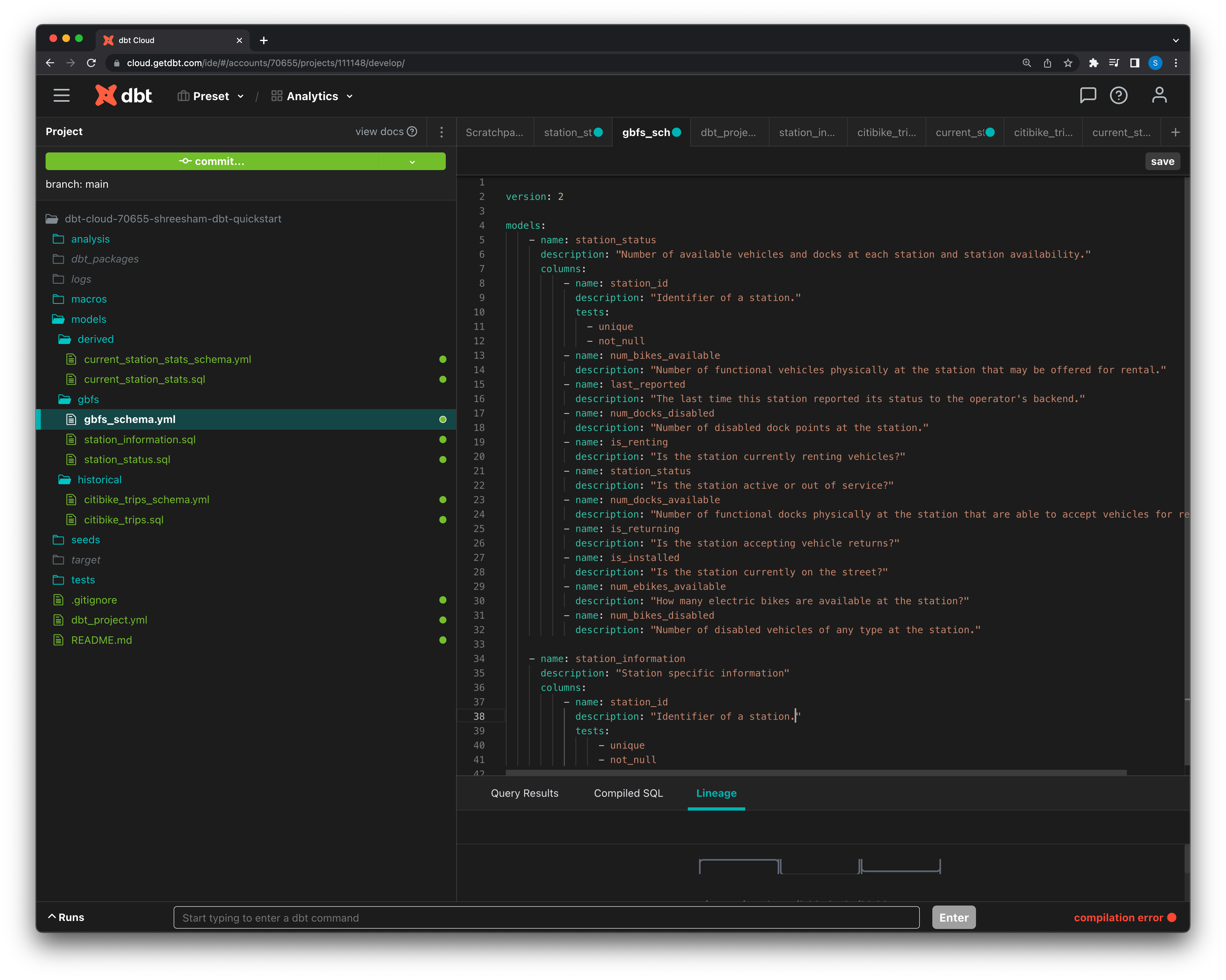
Here we’ve created a GBFS directory where we define the schemas of our feed models in a single YAML file and have the SQL files that dbt will run against our database to extract and load the two feeds we need — station_information and station_status.

Extract from JSON

-- station_status.sql for extraction and modeling as a table in Snowflake

{{ config(materialized='incremental') }}

with station_status_raw as (

    select
        t.value:"num_bikes_available",
        t.value:"last_reported",
        t.value:"num_docks_disabled",
        t.value:"station_id",
        t.value:"is_renting",
        t.value:"station_status",
        t.value:"eightd_has_available_keys",
        t.value:"num_docks_available",
        t.value:"is_returning",
        t.value:"is_installed",
        t.value:"num_ebikes_available",
        t.value:"legacy_id",
        t.value:"num_bikes_disabled"    
    from @station_status_stage/station_status.json,
    lateral flatten(parse_json($1):data.stations) as t

)

select 
    *
from station_status_raw

Depending on your underlying tools, the way the extraction is performed will be different. In Snowflake we have the raw JSON files staged, and we use a JSON parsing method as well as a Snowflake specific function to flatten the array data that’s parsed. The associated YAML file with the SQL file is what explicitly tells dbt what the schema of the new table to be created should be.
(station_status and station_information are extracted exactly the same way, the only difference being the data/schemas of the two.)

Derived Dataset Creation

{{ config(materialized='incremental') }}

with 
    /* 
        Store the current values of the derived table as a CTE using 'this' keyword.
        This is done for clarity in this example, we can also use 'this' to directly access the value
        in our total_current_rides CTE farther down.

        Necessary because the total rides value is what will update, which is why this 
        table is being materialized as an incremental table.

        'this' can be thought of as equivalent to ref('<the_current_model>'), 
        and is a neat way to avoid circular dependencies.
    */
    temp_current_state as (
        select *
        from {{ this }}
    ),
    historical_total_rides_by_station as (
        select
            count(ride_id) as total_rides,
            start_station_id,
            start_station_name
        from {{ ref('citibike_trips') }}
    ),
    /*
        We calculate the total number of rides by using the capacity 
        of the station from station info and subtracting the number of 
        available bikes at the station from station status data.
        Then we sum that back to the value we already had by using the
        values from the first CTE. 
    */
    total_current_rides as (
        select
            station_status.last_reported as last_updated_timestamp 
            temp_current_state.total_rides + historical_total_rides_by_station.total_rides + (station_information.capacity - station_status.num_bikes_available) as total_rides
        from {{ ref('station_information') }}, {{ ref('station_status') }}
        where 
            temp_current_state.start_station_id = historical_total_rides_by_station.start_station_id
            and temp_current_state.start_station_id = station_information.start_station_id
            and temp_current_state.start_station_id = station_status.station_id 
    )

select
    temp_current_state.start_station_name as start_station_name,
    temp_current_state.start_station_id as start_station_id,
    total_current_rides.total_rides as total_rides,
    total_current_rides.last_updated_timestamp as last_updated

From above, we know the historical data is provided to us with many of the dataset centric philosophies in mind specifically to be useful for visualization and analysis. All we need to do is reference that historical data and update it with the GBFS data to be able to visualize beyond the last day of the previous month!

Since we modeled in the station_information and station_status data, the last thing to do is to aggregate the GBFS station data as it comes in to create the derived dataset with the added aggregate calculations.

We calculate the number of rides from a station simply by using the capacity of the station (from station_information) and subtracting the number of available bikes (from station_status), incrementing our running total by that value, updating our last_updated_timestamp column with the station_status last_reported value, and we’re done!

Why in the transformation layer?

So why not simply surface the GBFS data as datasets and use the logic in the data viz layer?

Most importantly, the transformation layer already contains complexity managed with software development best practices:

• logic can be stored in source control
• data lineage can be understood and visualized
• change management like CI/CD hooks and automated testing becomes available

By moving the logic of the derived dataset out of the semantic layer (which is usually in the BI tool) and incorporating it in our transform layer with dbt’s ELT oriented approach we gain all of these advantages!

The second crucial benefit of this approach is that the datasets coming from the transform layer can be re-used by all of the data tools currently in use by you or your organization (ranging from R/Python notebooks, BI tools, data apps, etc).

Datasets should offer a simple and safe "dimensional" playground. By using the dataset-centric approach all charts built from these datasets can contain comprehensive relevant dimensions and metrics which enable users to self-serve within that context.

• This is much better than a “one-query-one-chart” approach where any sort of further analysis requires going back to the query and understanding it, understanding the underlying datasets, and then altering it to fit further questions.
• It’s also better than storing all logic in the semantic layer because the semantics can be progressively added over time to the transform layer in an agile way, instead of requiring a massive up-front definition.