Visualizing Dremio Workloads Using Preset Cloud

Dremio is a popular lakehouse platform that combines the best of data warehouses and data lakes. As Dremio usage increases in an organization, it becomes essential to understand the different workloads that are being run on the Dremio platform.

Metrics on Dremio workloads can help with monitoring your data platform, forecasting failures, adopting the platform, proactively addressing challenges that users might be facing, reducing total cost of the data platform ownership, and much more. While Dremio collects extensive data on workloads, the data isn’t available for querying out of the box.

In this article, we will go over some major key points where the data can be found, how to interpret certain data elements, and how to visualize key metrics using this data.

Data Sources

Dremio provides workload information in two data sources: queries.json and query profiles.

• Query Logs , also known as queries.json, contains high-level information on all queries that Dremio processed including ODBC, JDBC, UI, API, and Arrow Flight. The information in this file is sufficient to get metrics on query execution time, workload management queue the query was assigned to, datasets that query was using, etc. This file can also be used for audit trail purposes. However, the queries.json does not provide any detailed information on query execution.
• For detailed information on query execution, the Dremio UI provides a Job UI page, also known as Query Profile. The Job UI provides detailed information on query execution broken down by phases, threads, and operators. The query profile in the Job UI is usually utilized for query optimization. However, aggregating this data across queries will produce valuable information about the workload and the infrastructure. For example, increased wait time indicates hitting a bottleneck in some resource, such as overwhelmed storage or oversubscribed CPU.

Data Acquisition

Dremio generates the queries.json file in the coordinator’s log directory along with other log files.

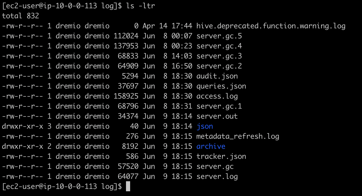
Dremio follows the same file rotation strategy that it uses for the rest of the log files and keeps a limited history of it in the archive sub-directory. Since Dremio Executors cannot consume data from the coordinator’s log directory, Dremio cannot query queries.json files out of the box. The data must be residing in a storage accessible by all executors, such as an S3 bucket or HDFS.

Dremio follows the same file rotation strategy that it uses for the rest of the log files and keeps a limited history of it in the archive sub-directory. Since Dremio Executors cannot consume data from the coordinator’s log directory, Dremio cannot query queries.json files out of the box. The data must be residing in a storage accessible by all executors, such as an S3 bucket or HDFS.

It’s easy to set up a cron job to copy the queries.json file and the archived files on a regular basis to a data storage system of your choice and make it available for querying. For AWS implementations we recommend using AWS sync command, for EKS implementations it could be done with an additional container as in this Helm Chart.

Query profiles can be downloaded from the Job UI manually or automatically via an undocumented Dremio API. However, since this API is not documented, it’s a subject to change without notice and the more reliable way is to use the Dremio-admin CLI to extract query profiles in batches.

Query profiles are zip files. The file names represent the Job Id. Each file includes several json files such as header.json and profile_attempt_0.json. The number of embedded files depends on whether Dremio had to attempt to execute the query more than once and if a prepared statement approach was used.

Unlike queries.json, query profiles need some transformation before they can be utilized for querying by Dremio. One such transformation is adding a jobId as a field inside each JSON file. After that, these files can be copied over to a distributed storage for querying as JSON files or transformed into parquet files.

Using Query Logs

Dremio provides some documentation on the queries.json file, covering only a few fields. This file contains a lot of useful information and below is a complete list of attributes at the time of writing this article:

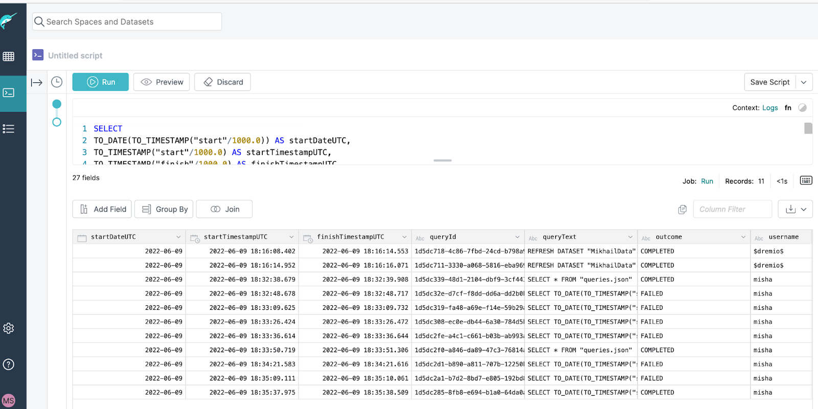
Below is an example of SQL query that you can run against queries.json.

SELECT
TO_DATE(TO_TIMESTAMP("start"/1000.0)) AS startDateUTC,
TO_TIMESTAMP("start"/1000.0) AS startTimestampUTC,
TO_TIMESTAMP("finish"/1000.0) AS finishTimestampUTC,
queryId,
queryText,
outcome,
username,
inputRecords,
inputBytes,
outputRecords,
outputBytes,
requestType,
queryType,
CONVERT_FROM(parentsList, 'JSON') parentsList,
queryCost,
queueName,
accelerated,
outcomeReason,
schema,
poolWaitTime AS poolWaitTimeMs,
pendingTime AS pendingTimeMs,
metadataRetrievalTime AS metadataRetrievalTimeMs,
planningTime AS planningTimeMs,
engineStartTime AS engineStartTimeMs,
queuedTime AS queuedTimeMs,
executionPlanningTime AS executionPlanningTimeMs,
startingTime AS startingTimeMs,
runningTime AS runningTimeMs,
“finish” - "start" AS durationMs
FROM “queries.json”

The result of that sample query may look like this:

JSON files packaged within the query profile zip file do not have Job ID which is required to join to queries.json. Job ID is also a crucial bit of information if you want to find this particular query in Dremio UI. Luckily, the query profile zip file name represents Dremio Job ID. For example, “90c316e0-8093-4ced-aaed-87befaf16ea2.zip” file was used to produce the screenshot above. With that, the Job ID can be extracted from the file name and can be used to populate the datasets during transformation into parquet.

Organizing Dremio Workload Analytics

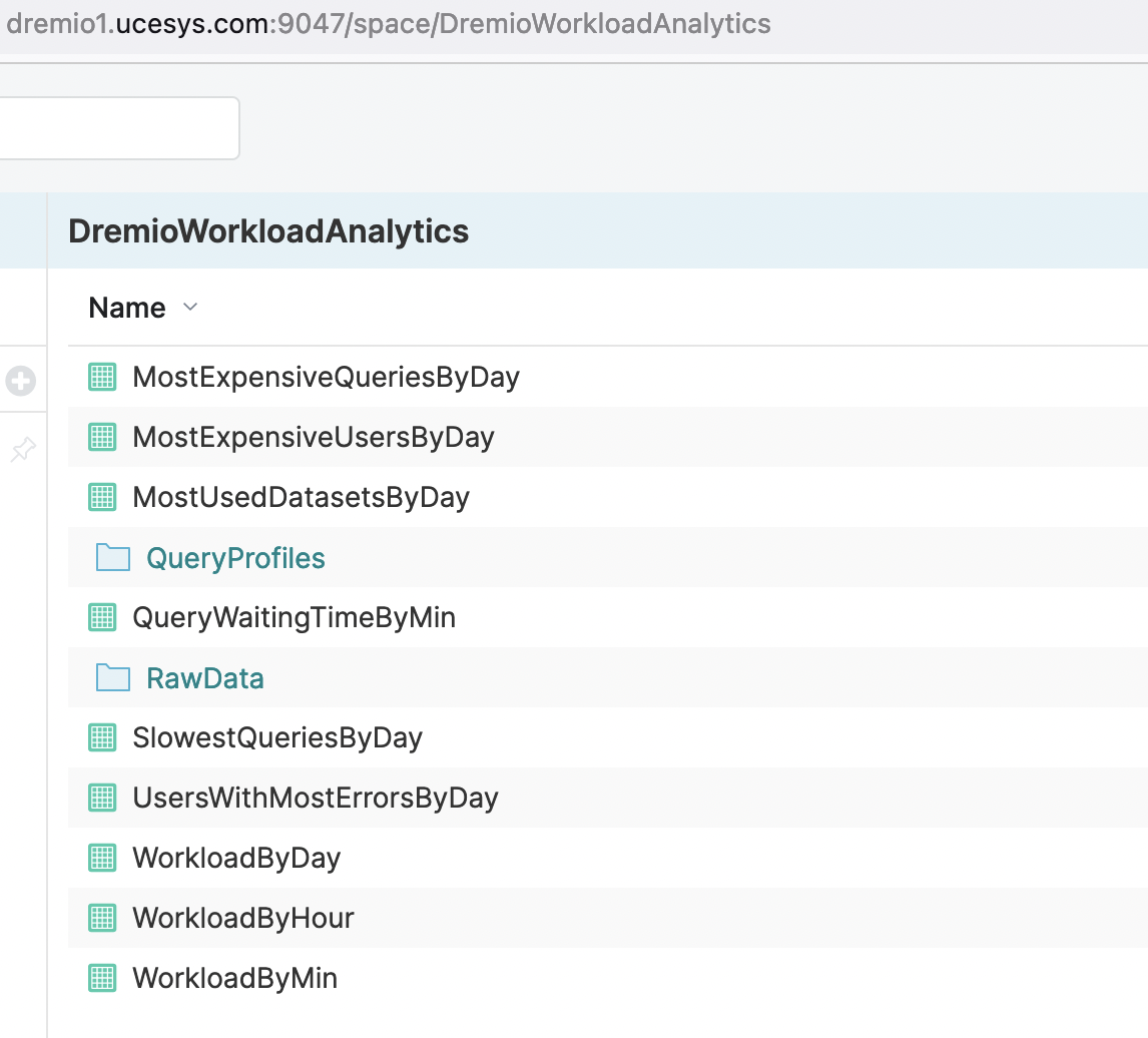
One of the ways to organize virtual datasets in Dremio for different teams to access them is to create a dedicated space (e.g. named DremioWorkloadAnalytics). This space can contain all the analytical VDS as well as Raw and Prep layers as you can see in a screenshot below:

Visualizing Dremio Workload Analytics

Next, let's get a tour of the insights you can gain from visualizing Dremio workloads in Preset Cloud.

Setting up a A Dashboard in Preset

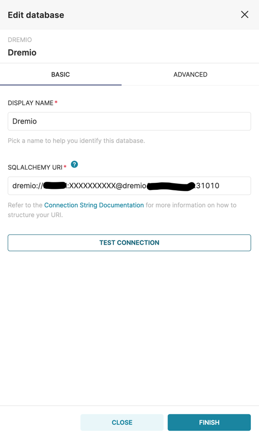
Let’s assume that we’re analyzing this particular Dremio installation for the first time. As a start it would be nice to understand typical workload to be able to address most common performance challenges. Preset Cloud supports Dremio out of the box. The first step is to enter the Add Database screen from within a Preset workspace:

As soon as connection to Dremio is established we need to register datasets that we will be using for this article. We will build our dashboard using 2 datasets with different time grain:
timestamp-grain dataset for workload overview and detailed view of High SLA queries performance;
weekday and hour dataset with averaged values for most of the charts.

To register a dataset in Preset, click Add Dataset and select the Virtual Datasets that we created in Dremio.

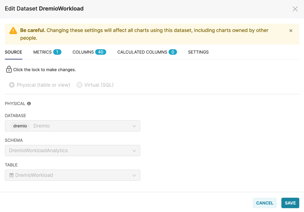
As soon as datasets are registered in Preset, we can start visualizing the data. Preset has plenty of chart types that are covering most of the use cases. To create a new chart, you need to specify registered dataset that will feed the data in and choose the chart type:

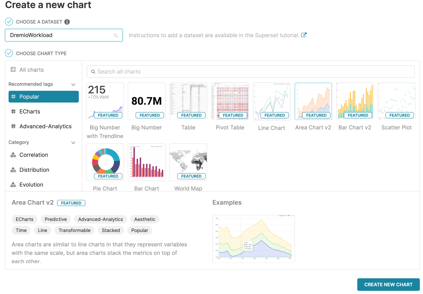
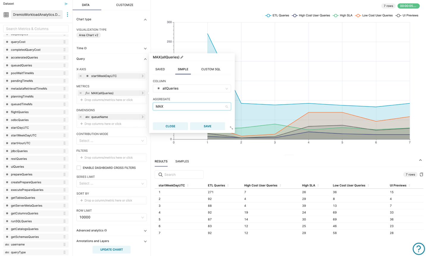
Now you can start configuring the chart specifying dimensions, metrics and other parameters. Please refer to the Preset documentation for more information on creating charts.

Basic Charting

Let’s start by charting some basic metrics from the data:

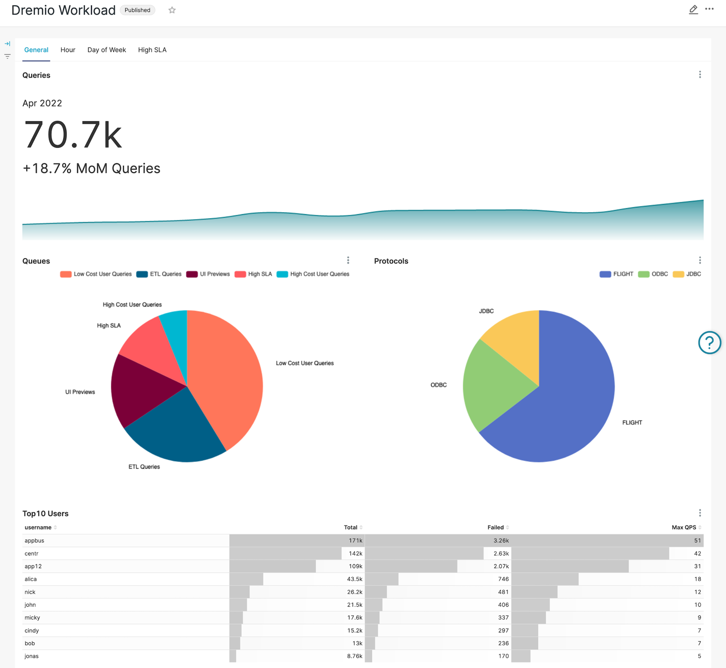
The topmost chart is a visualization of the overall number of queries Dremio has processed over the last year. The workload illustrates a fairly steady increase in the number of queries over the year with a couple of minor dips.

Distribution of queries across different Dremio workload management queues seems pretty normal and does not raise any concerns. However, we can see the first anomaly in protocol distribution: while UI Preview queue weighs almost 17% of the workload, the REST protocol is not used at all, and we can happily start discussion with application frontend team since modern approach to frontend application development assume on-demand data loading techniques with REST protocol usage.

Another interesting (and positive!) observation is high utilization of Apache Arrow Flight protocol. Roughly 65% of the workload is using this high-performance protocol which is many times faster than ODBC or JDBC.

At the bottom of the General tab, we have placed a user scoreboard with total number of queries executed, total number of failed queries, as well as the maximum QPS (queries per second) – it’s always valuable to understand what your users are up to!

Apart from the relatively high number of failed queries for top users, an eye-catching finding is that runner-ups are having somewhat disproportionally high QPS rate (queries per second). It might be worth deeper investigation since it could happen that they are bursting the system with failing queries potentially affecting other users. To address workload isolation, we might also consider creating a separate queue for this kind of workload.

Analyzing Hourly Workload

Moving on to the “hour of the day” view. This type of workload analytics will give us good understanding of typical shape of our daily workload:

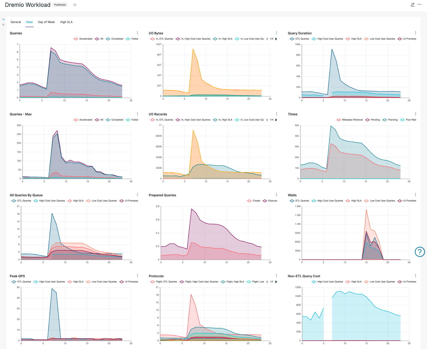
The Queries chart seems pretty natural, given the ETL jobs are running overnight. Successfully completed query rate also looks good, slightly decreasing during office hours. What draws attention is the dramatically low number of accelerated queries. This means that we are not gaining benefits of Dremio Reflections – the cornerstone of Dremio performance acceleration. We need to address this issue for sure by carefully investigating usage patterns and creating row and aggregate Dremio Reflections to boost productivity, decrease system workload and reduce operational costs.

Max Queries chart looks similar to the one with average values, however it’s worth noting that while it seems like overnight ETL workload has little deviation, 7-8am workload peak is way higher than you might expect since the workday starts about the same time. Cross-checking this peak with All Queries by Queue chart shows that this is due to the ETL workload, probably still running its final steps. All Queries By Queue charts prove the theory – with a peak of ETL workload during the same time. It might be worth moving the 7am ETL workload to earlier time since regular users (Low Cost User Queries and UI Previews queues) start their daily activities before the ETL workload is completed. Besides obvious performance issues, it could potentially lead to data quality issues and incorrect business reporting since the ETL might not have finished preparing the data.

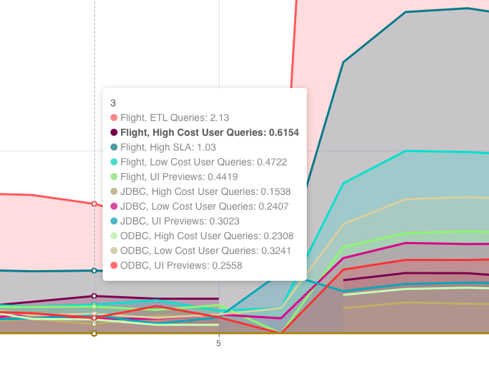
Another anomaly is the dead period in the High Cost SLA queue between 5 and 7am. We can see the same issue in the Query Duration and the Non-ETL Query Cost charts as well. The Protocol chart provides a bit more information: this gap is related to the High-Cost User Queries workload that uses Arrow Flight protocol. It’s definitely worth digging deeper to understand what’s going on and monitor system behavior during that time.

It would be intuitive to expect that the number of “prepare statement” requests should be a bit lower than the number of times these “prepared” statements were utilized for actual query execution. However, as per the Prepared Queries chart we observe exactly opposite. That could indicate potential implementation issues or even bugs in the client systems. For example, queries might get prepared, but never executed for some reason.

In the chart below we observe an interesting anomaly – a spike of “waiting time” that starts at approximately 3pm and lasts till 6pm daily. High waiting time is an indication of resource contention in Dremio, either CPU or I/O. It usually leads to abnormally slow performance. From our experience, the root cause usually could be found in over-utilized or failing hardware. It’s worth checking on other heavy processes sharing nodes and other resources with Dremio. This anomaly needs to be investigated further with proper RCA as soon as possible.

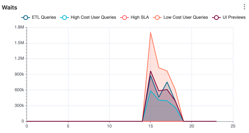
Another observation worth investigating is the presence of ETL queries during business hours. Since there is a correlation with increased waiting time it might be a good starting point for root cause analysis of the waiting time anomaly.

Weekly View

And now let’s step back and observe Dremio workload from heights of the weekly perspective:

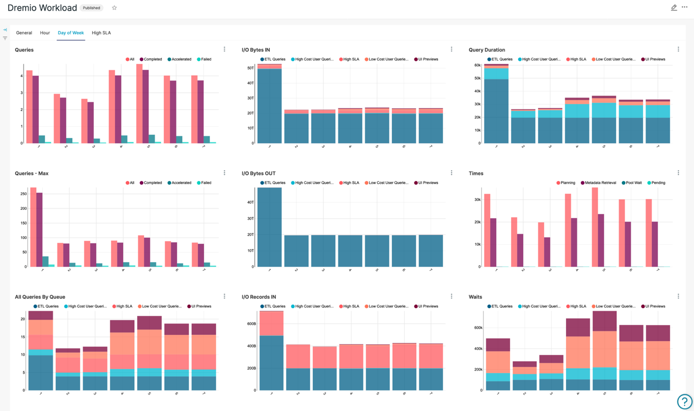
This level of aggregation is useful in reviewing the overall system health and distribution of heavy-weight jobs over time.

Expected observation is that Sunday is the busiest data lifting day. Sunday workload is probably the heaviest weekly ETLs workload from the perspective of number of queries, QPS, and I/O.
Quick check of query timings indicates that the overall system is healthy during the ETL processes, probably due to low interactive user workload.

Another finding is that the workload looks a bit lower on Mondays and Tuesdays. As such, these days might be good candidates for future heavy analytical workload.

Monitoring SLA

Performance monitoring is very important for High SLA workload. Let’s set up a chart to review High SLA workload performance and our SLA compliance.

To do so, we need to produce visualization of average and peak values of Query Duration for High SLA workload management queue:

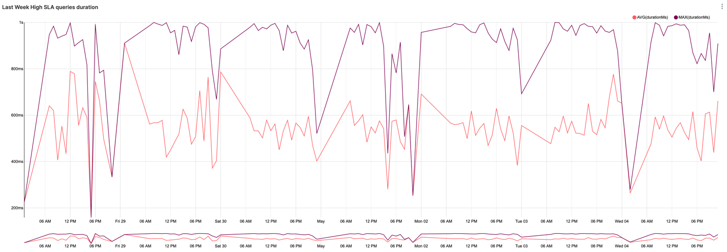
Assuming sub-second SLA, we can conclude that we’re meeting SLA so far. However, the peak query duration reaching our SLA limits alarms us that outliers can potentially start going beyond the SLA limits since the overall Dremio workload tends to grow over time as we can see from the General tab. Further detailed investigation and taking preventative measures would be a good idea.

Conclusion

Proper Dremio Monitoring is very important for providing a stable and reliable analytical data platform. Dremio provides data for monitoring in various ways. In this article we touched on Workload Analysis which is important for understanding your workload and its tendencies, an often overlooked aspect of the state of user adoption. While we covered some basic metrics and their interpretation it’s only a starting point. Many more metrics can be derived from the workload data provided by Dremio.

Besides the Workload data, Dremio provides data for monitoring via API, SQL, and JMX. We will try to cover Dremio Monitoring in the future articles.

About UCE Systems

UCE Systems is a high impact consulting company specializing in data platform and analytics. Our sharply focused expertise allows us to accurately identify our customers’ pain points and fine tune data platform to get the most value from your investments. Please contact us with any questions at ask@ucesys.com.