


Optimize Your Database for Dashboard Performance


Slow dashboards can be frustrating and remain an all too common problem when visualizing data in business intelligence tools. Modern BI tools like Apache Superset or Preset generate SQL queries on behalf of end-users by providing a no-code interface to build charts and visualizations, which makes data accessible to significantly more people. Everything has a trade-off though, and this also makes it easier to ignore the complexity of the steps needed to produce charts and dashboards. Slow loading or slow refreshing dashboards are often a motivating reason to better understand the queries your BI tool generates and how to set-up your database for success in serving and responding to those queries quickly.
There are typically three best practices to improve dashboard performance. From the most to least impactful they are:
- Optimizing your database for querying
- Enhancing your dashboard for viewing
- Improving access to your dashboard
In this post we’ll focus on the one with the greatest impact — optimizing your database for your queries. While the other two can have an impact, they are typically simpler to understand and implement in practice. Check out the Preset documentation on maximizing performance to learn more about these two categories!
Recommendations
Before we go into each of the concepts, here's a quick table with the concepts and a gist of the importance with implementation details:
| Concept | Why it’s important | How to implement |
|---|---|---|
| Summarized Materialized View/Table | Pre-calculated values reduce subsequent operations on the dataset | Utilizing a variety of tools such as Airflow or dbt, commonly-used joins and aggregations can be defined as materialized views or tables that can then be used in Preset as a Physical Dataset. |
| Partitioning | Eliminating data that is less relevant to the end user can reduce the time that the database spends scanning and computing | Break large datasets into partitions (such as by department or timeframe) based on access needs. Historical data can be aggregated while recent data can offer granular changes. Note that partitions are only useful where predicates (filters) are applied to the partition columns. This allows the database to perform “partition pruning” and limit scanning based on the predicate. |
| Indexing | Indexing minimizes scans required when a query is processed | Columns that are frequently used for filtering, such as time or a particular category, should be used for indexing the dataset. |
| Filtering | Filtering bounds data scans to reduce the data compute | Add filters to your query or apply a WHERE clause when creating your dataset to reduce irrelevant data for the end user. |
Summarized Materialized View or Table
Materialized views are used in databases to increase the speed of queries on very large databases. Querying large databases often involve joins between tables, the use of aggregations (such as SUM, MAX, etc.), or both. These operations are very expensive in terms of time and processing power — which is why you want to avoid having too many of these created through the use of virtual datasets in Preset as that can substantially slow down your dashboarding experience.
Materialized views in the database improve query performance by pre-calculating time consuming join and aggregation operations on the database prior to execution time and storing the results in the database. Once a new table or view is created with these pre-calculated operations, it can be accessed directly as a physical dataset in Preset. Virtual dataset queries (specifically for last-mile light transformations/computations) can now be directed to the materialized view and not to the underlying detail tables. You can utilize a variety of tools, pre-viz layer, like Airflow or dbt to perform these commonly-used joins and aggregations and create the materialized views you need.
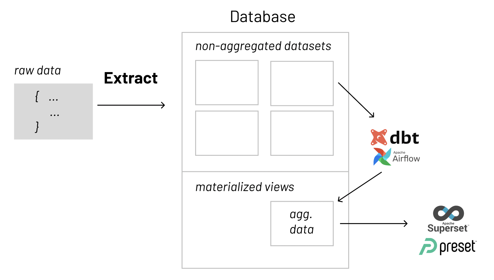
To summarize — in databases, materialized views (or tables) can be used to pre-calculate and store aggregated data such as the sum of sales. Materialized views in these environments are typically referred to as summaries, because they store summarized data. They can also be used to pre-calculate joins with or without aggregations. A materialized view eliminates the overhead associated with expensive joins or aggregations for a large or important class of queries.
Partitioning
Partitioning is a process where very large tables are divided into multiple smaller parts within your database. By splitting a large table into smaller, individual tables, queries that access only a fraction of the data can run faster because there is less data to scan. The main of goal of partitioning is to aid in maintenance of large tables and to reduce the overall response time to read and load data for particular SQL operations.
Vertical Partitioning
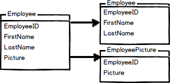
Vertical table partitioning is mostly used to increase database performance especially in cases where a query retrieves all columns from a wide table that contains a large number of columns. In this case to reduce access times the columns of that table can be split to create their own tables. Another example is to restrict access to sensitive data e.g. passwords, salary information etc. Vertical partitioning splits a table into two or more tables containing different columns:
Horizontal Partitioning
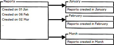
Horizontal partitioning divides a table into multiple tables that contain the same number of columns, but fewer rows. For example, if a table contains a large number of rows that represent monthly reports it could be partitioned horizontally into tables by years, with each table representing all monthly reports for a specific year. This way queries requiring data for a specific year will only reference the appropriate table. Tables should be partitioned in a way that queries reference as few tables as possible.
Tables are horizontally partitioned based on a column which will be used for partitioning and the ranges associated to each partition. Partitioning column is usually a datetime column but all data types that are valid for use as index columns can be used as a partitioning column, except a timestamp column.
Indexing
Indices are a powerful tool used in the background of a database to speed up querying. Indices power queries by providing a method to quickly lookup the requested data.
Simply put, an index is a pointer to data in a table. An index in a database is very similar to an index in the back of a book.
Why are indices needed?
Imagine walking into the Library of Congress and being given the task to find a specific publishing within 10 minutes. Would you be able to complete this task within the given time frame? The Library of Congress is considered the largest library in the world and it houses approximately 170 million items. Intuitively, we know this isn’t much of a challenge. The first thing we would do is ask for access to the library’s index because indices contain all the necessary information needed to access items quickly and efficiently.
Similarly, a database index contains all the necessary information to access data quickly and efficiently. Big data is everywhere today, with companies processing several hundred petabytes (1000⁵ bytes) of data per day. Storing all of this data in a database is great, but for a data company, being able to access that data efficiently is paramount to success. Just like the Library of Congress example, one way of solving the access issue when it comes to large amounts of data is through the use of indices. Indices serve as lookup tables that efficiently store data for quicker retrieval.
How are indices created?
In a database, data is stored in rows which are organized into tables. Each row has a unique key which distinguishes it from all other rows and those keys are stored in an index for quick retrieval.
Since keys are stored in indices, each time a new row with a unique key is added, the index is automatically updated.
However, sometimes the need to quickly lookup data that is not stored as a key comes up. For example, we may need to quickly lookup customers by phone number. It would not be a good idea to use a unique constraint because we can have multiple customers with the same phone number. In these cases, we can create our own indices.
The syntax for creating an index will vary depending on the database. However, the syntax typically includes a CREATE keyword followed by the INDEX keyword and the name we’d like to use for the index. Next should come the ON keyword followed by the name of the table that has the data we’d like to quickly access. Finally, the last part of the statement should be the name(s) of the columns to be indexed.
CREATE INDEX <index_name>
ON <table_name> (column1, column2, ...)
For example, if we would like to index phone numbers from a customers table, we could use the following statement:
CREATE INDEX customers_by_phone
ON customers (phone_number)
The users cannot see the indices, they are just used to speed up searches/queries.
Note*:** Updating a table with indices takes more time than updating a table without (because the indices also need an update). So, only create indices on columns that will be frequently searched against.*
OLAP vs OLTP Databases
Before data can be put to use, it must be processed. Online analytical processing (OLAP) and online transactional processing (OLTP) are the two primary data processing systems used. OLAP is designed to analyze multiple data dimensions at once, helping teams better understand the complex relationships in their data. This system is ideal for uncovering valuable business insights. OLTP is a simple transactional system ideal for handling online transactions at scale. Although each one’s purpose and method of processing data are different, OLAP and OLTP systems are both valuable for solving complex business problems.
The main distinction between OLAP vs. OLTP is the core purpose of each system. An OLAP system is designed to process large amounts of data quickly, allowing users to analyze multiple data dimensions in tandem. Teams can use this data for decision-making and problem-solving.
In contrast, OLTP systems are designed to handle large volumes of transactional data involving multiple users. Relational databases rapidly update, insert, or delete small amounts of data in real time. Most OLTP systems are used for executing transactions such as online hotel bookings, mobile banking transactions, e-commerce purchases, and in-store checkout. Many OLAP systems pull their data from OLTP databases via an ETL pipeline and can provide insights such as analyzing ATM activity and performance over time.
Simply put, organizations use OLTP systems to run their business while OLAP systems help them understand their business.
The table below summarizes some of the main differences between the two:
| Parameters | OLAP | OLTP |
|---|---|---|
| Backup and Recovery | OLAP systems require backup less frequently. | Backup and recovery are the polar opposite when witnessed from the perspective of an OLTP system. A complete backup at any moment in time is mandatory along with some kind of provision for incremental backups. |
| Data | It makes use of the data warehouse concept and is an online database query management system. | Relies on traditional database management systems. |
| Data Integrity | OLAP systems go through infrequent transactions. Hence, OLAP systems don’t necessarily require for data integrity. | Data integrity can’t be ignored when OLTP systems are concerned as the OLTP system frequently executes transactions that modify the database. |
| Primary Intent | OLAP system allows the user to retrieve/extract multidimensional data that can be analyzed and used for decision making. | OLTP system focuses on inserting, updating, and sometimes deleting information from the database |
| Storage Space Requirements | OLAP systems ask for significant storage space due to the existence of aggregation structures and historical data. | It requires smaller storage space and even smaller space for those systems with archived historical data. |
| System Type | OLAP is an online data retrieval and analysis system. | OLTP is an online transaction system. |
| Transactions | Transactions much longer but the frequency is more. | Short and fast, but the frequency of transactions is less. |
| Query Complexity | Complex queries | Simple queries |
| Audience | Customer-oriented | Market-oriented |
| Table | Tables are not normalized | Tables are normalized |
| Response time | In seconds to minutes | In milliseconds |
Back to Indexing!
When deciding how to index your data base, typically speaking, you want to keep your OLTP system sleek and fast. The more indices put on an OLTP table, the slower all insert, update, and delete statements become. This can cause “overhead locking” until the transaction is complete and possibly slow down other queries or users interacting with the same tables.
OLAP database have less constraints for response time. It is generally acceptable for an OLAP database to run slower than an OLTP database. Typically there are either massive non-transactional updates and/or massive non-transactional queries hitting OLAP databases.
To summarize indices in an OLAP/OLTP context:
- Less indices on an OLTP database will result in less locks and faster response due to less entities that have to be modified on an insert, update, or delete.
- Extra indices in an OLAP environment are not as important because the response time for the return of the result set should have a longer expectation.
And to summarize indexing for databases in general:
- Indices are a powerful tool used in the background of a database to speed up querying.
- Indices contain all the necessary information needed to access items quickly and efficiently.
- Indices serve as lookup tables to efficiently store data for quicker retrieval.
- Table keys are stored in indices.
- Indices for non-key values can be created with a
CREATE INDEXstatement.
Filtering
Three common options for storage are text files, spreadsheets, and databases. Text files are easiest to create, and work well with version control, but then we would have to build search and analysis tools ourselves. Spreadsheets are good for doing simple analyses, but they don’t handle large or complex data sets well. Databases, however, include powerful tools for search and analysis, and can handle large complex data sets.
One of the most powerful features of a database is the ability to filter data, i.e., to select only those records that match certain criteria.
About the Data
In the late 1920s and early 1930s, William Dyer, Frank Pabodie, and Valentina Roerich led expeditions to the Pole of Inaccessibility in the South Pacific, and then onward to Antarctica. In 2015, their expeditions were found in a storage locker at Miskatonic University.
Back to Filtering!
For example, suppose we want to see when a particular site was visited. We can select these records from the Visited table by using a WHERE clause in our query:
SELECT * FROM Visited WHERE site = 'DR-1';| id | site | dated |
|---|---|---|
| 619 | DR-1 | 1927-02-08 |
| 622 | DR-1 | 1927-02-10 |
| 844 | DR-1 | 1932-03-22 |
The database manager executes this query in two stages. First, it checks at each row in the Visited table to see which ones satisfy the WHERE. It then uses the column names following the SELECT keyword to determine which columns to display.
This processing order means that we can filter records using WHERE based on values in columns that aren’t then displayed:
SELECT id FROM Visited WHERE site = 'DR-1';| id |
|---|
| 619 |
| 622 |
| 844 |

We can use many other Boolean operators to filter our data. For example, we can ask for all information from the DR-1 site collected before 1930:
SELECT * FROM Visited WHERE site = 'DR-1' AND dated < '1930-01-01';| id | site | dated |
|---|---|---|
| 619 | DR-1 | 1927-02-08 |
| 622 | DR-1 | 1927-02-10 |
If we want to find out what measurements were taken by either Lake or Roerich, we can combine the tests on their names using OR:
SELECT * FROM Survey WHERE person = 'lake' OR person = 'roe';| taken | person | quant | reading |
|---|---|---|---|
| 734 | lake | sal | 0.05 |
| 751 | lake | sal | 0.1 |
| 752 | lake | rad | 2.19 |
| 752 | lake | sal | 0.09 |
| 752 | lake | temp | -16 |
| 752 | roe | sal | 41.6 |
| 837 | lake | rad | 1.46 |
| 837 | lake | sal | 0.21 |
| 837 | roe | sal | 22.5 |
| 844 | roe | rad | 11.25 |
Alternatively, we can use IN to see if a value is in a specific set and obtain the same results as above:
SELECT * FROM Survey WHERE person IN ('lake', 'roe');| taken | person | quant | reading |
|---|---|---|---|
| 734 | lake | sal | 0.05 |
| 751 | lake | sal | 0.1 |
| 752 | lake | rad | 2.19 |
| 752 | lake | sal | 0.09 |
| 752 | lake | temp | -16 |
| 752 | roe | sal | 41.6 |
| 837 | lake | rad | 1.46 |
| 837 | lake | sal | 0.21 |
| 837 | roe | sal | 22.5 |
| 844 | roe | rad | 11.25 |
We can combine AND with OR, but we need to be careful about which operator is executed first. If we don’t use parentheses, we get this:
SELECT * FROM Survey WHERE quant = 'sal' AND person = 'lake' OR person = 'roe';| taken | person | quant | reading |
|---|---|---|---|
| 734 | lake | sal | 0.05 |
| 751 | lake | sal | 0.1 |
| 752 | lake | sal | 0.09 |
| 752 | roe | sal | 41.6 |
| 837 | lake | sal | 0.21 |
| 837 | roe | sal | 22.5 |
| 844 | roe | rad | 11.25 |
which is salinity measurements by Lake, and any measurement by Roerich. We probably want this instead:
SELECT * FROM Survey WHERE quant = 'sal' AND (person = 'lake' OR person = 'roe');| taken | person | quant | reading |
|---|---|---|---|
| 734 | lake | sal | 0.05 |
| 751 | lake | sal | 0.1 |
| 752 | lake | sal | 0.09 |
| 752 | roe | sal | 41.6 |
| 837 | lake | sal | 0.21 |
| 837 | roe | sal | 22.5 |
We can also filter by partial matches. For example, if we want to know something just about the site names beginning with “DR” we can use the LIKE keyword. The percent symbol acts as a wildcard, matching any characters in that place. It can be used at the beginning, middle, or end of the string:
SELECT * FROM Visited WHERE site LIKE 'DR%';| id | site | dated |
|---|---|---|
| 619 | DR-1 | 1927-02-08 |
| 622 | DR-1 | 1927-02-10 |
| 734 | DR-3 | 1930-01-07 |
| 735 | DR-3 | 1930-01-12 |
| 751 | DR-3 | |
| 752 | DR-3 | 1930-02-26 |
| 844 | DR-1 | 1932-03-22 |
Finally, we can use DISTINCT with WHERE to give a second level of filtering:
SELECT DISTINCT person, quant FROM Survey WHERE person = 'lake' OR person = 'roe';| person | quant |
|---|---|
| lake | sal |
| lake | rad |
| lake | temp |
| roe | sal |
| roe | rad |
But remember: DISTINCT is applied to the values displayed in the chosen columns, not to the entire rows as they are being processed.
This expedition data came from Software Carpentry’s repo if you’re interested in seeing some of the other data!
Native Dashboard Filters in BI Tools
The impact of filtering and its impact on the speed of query execution is often neglected. As we mentioned earlier, many modern BI tools generate SQL queries on behalf of end-users by providing no-code interfaces to build charts. Data becomes more accessible to a wider audience as a result, but, as the audience grows the general technical level of the audience decreases. A curated/pre-filtered dataset may not always be available directly from the database level for what the data consumers are doing at the moment.
Below is an example in Preset where using the built in filter configuration demonstrates the impact on the speed of the auto-generated query needed to create the chart!
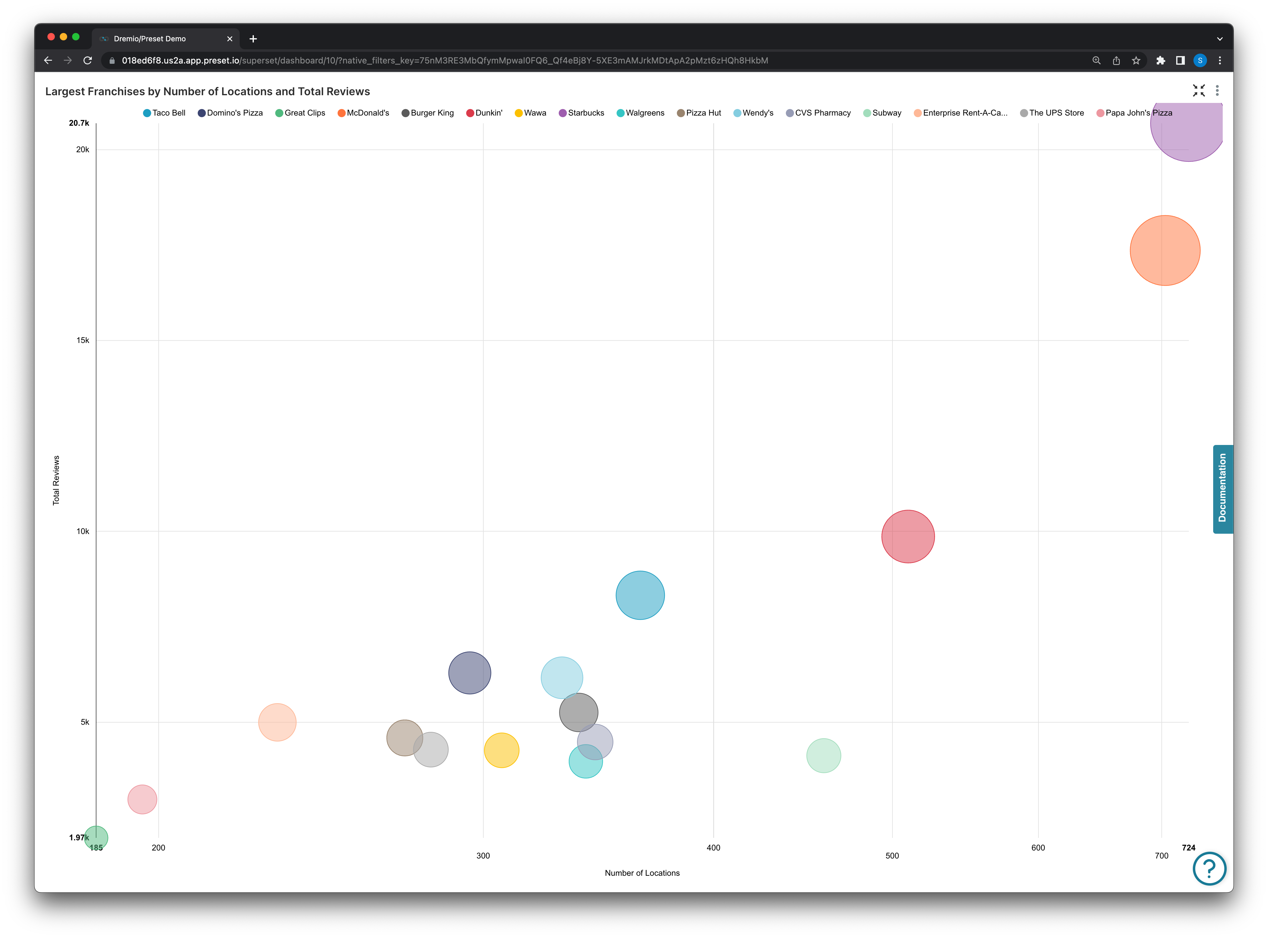
A bubble chart is used to visualize a metric across three dimensions of data in a single chart (X-axis, Y-axis, and bubble size). The bubble chart below was created from Yelp’s open dataset to place bubbles sized by the number of reviews that franchise had, with the X-axis being the total number of locations that had been reviewed, and the Y-axis simply being the count of total reviews for a franchise (franchise defined here as a business with a unique business_id but the same name as at least one other business).
SELECT name AS name,
       max(total_reviews) AS "MAX(total_reviews)",
       sum(num_locations) AS "SUM(num_locations)",
       sum(total_reviews) AS "SUM(total_reviews)"
FROM
  (with franchises as
     (SELECT name,
             COUNT(distinct business_id) as num_locations
      FROM "Curated Data"."Business + Yelp Reviews"
      GROUP BY name),
        franchise_and_reviews as
     (select distinct business_id,
                      name,
                      review_count
      from "Curated Data"."Business + Yelp Reviews"),
        fr_review_sum as
     (SELECT name,
             sum(review_count) as total_reviews
      FROM franchise_and_reviews
      GROUP BY name) SELECT f.name,
                            f.num_locations,
                            frs.total_reviews
   FROM franchises f,
        fr_review_sum frs
   WHERE f.name = frs.name
     and f.num_locations > 1) AS virtual_table
WHERE num_locations >= 185
GROUP BY name
From the generated query above we can see we configured the filter to only look for franchises with greater than or equal to 185 locations:
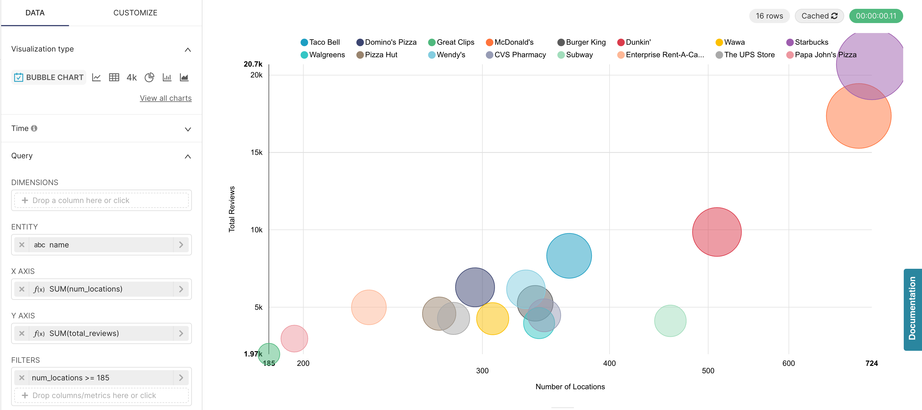
This generated query took 0.11 seconds (green button in the top right) to run and create the visualization.
Now we altered that filter to look for greater than or equal to 100 locations:
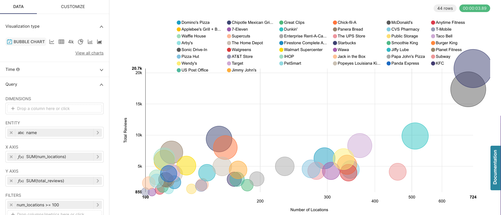
From above we can see that changing the filter to include more small franchises caused the generated query to run for 3.89 seconds a whopping 35 times longer, with the only change being the filter, reflected by the change in the last WHEREclause of the generated query below:
SELECT name AS name,
       max(total_reviews) AS "MAX(total_reviews)",
       sum(num_locations) AS "SUM(num_locations)",
       sum(total_reviews) AS "SUM(total_reviews)"
FROM
  (with franchises as
     (SELECT name,
             COUNT(distinct business_id) as num_locations
      FROM "Curated Data"."Business + Yelp Reviews"
      GROUP BY name),
        franchise_and_reviews as
     (select distinct business_id,
                      name,
                      review_count
      from "Curated Data"."Business + Yelp Reviews"),
        fr_review_sum as
     (SELECT name,
             sum(review_count) as total_reviews
      FROM franchise_and_reviews
      GROUP BY name) SELECT f.name,
                            f.num_locations,
                            frs.total_reviews
   FROM franchises f,
        fr_review_sum frs
   WHERE f.name = frs.name
     and f.num_locations > 1) AS virtual_table
WHERE num_locations >= 100
GROUP BY name
Dashboard filters are another good way to reduce the total data scanned to only what is needed and speed up dashboard performance, but the best optimization will always be to optimize by creating pre-calculated datasets at the database level to be used for visualization or analysis.
A Quick Disclaimer
It’s important to note that every database differs quite a bit in terms of the switches and levers that they expose for optimization purposes. Databases expose things like partitions, indices of a variety of shape, materialized views, different storage tiers, all in different ways — and that’s without speaking about the database specific technologies. If your database can process a large arbitrary dataset quickly regardless of tuning, then you don’t have to do much tuning and can expect decent response time on arbitrary workloads.
Nevertheless, creating pre-calculated and/or aggregated data views that align closely with your end user's visualization goals can reduce the run time of a query.
When in doubt, running an explain on your query can help you understand which operation is taking the longest time!
